The Doubling Cube
Janowski’s model, measured against 33,395 rolled-out equities — and what Raccoon will build from it.
Rick Janowski’s cube-life-index model is how a cubeless evaluation becomes a cube decision. GNU Backgammon and eXtreme Gammon both ship it, and its published constant — \(x = 0.68\) for contact positions — has stood essentially unchanged since 1993. It is rarely measured, because measuring it needs observed cubeful equities for a large and varied set of real positions.
Those observations were already on disk. The BGSage money benchmark rolled positions out to completion with the cube live, recording for each candidate a measured cubeful equity next to the cubeless probabilities for the same position — and the cube sits in a different place across them, which is what makes the model separable. This page tests it on 33,395 of those, then says exactly what Raccoon should implement.
The short answer is that the model is in good shape and the conventional constant survives. Two of the three equity formulas are correct at \(x = 0.68\) to within 0.018 of a point. The third, for a centred cube, wants a much higher index — but adopting it buys nothing where the parameter is actually read, and we cannot explain it, so we are not acting on it. What is worth fixing is structural: use the piecewise form, respect the provable bounds, and floor \(W\) and \(L\) at one point.
Two numbers this page used to report were wrong, and both errors are the same kind, so they are worth stating rather than quietly correcting. Reference quality is recorded in two fields, not one: filtering on eval_level alone admitted truncated rollouts whose leaves call Janowski. Against references that include them, retuning the index looks worth +1.167 ± 0.271 cube PR. Against references that are actually measurements it is worth +0.128 ± 1.242 — nothing. The measurement section sets out the filter that separates them.
Everything here is money play with the Jacoby rule and beavers on, matching the benchmark. Match play, where the score moves every take point, is out of scope and is not calibrated by anything below.
The model is three formulas
A network evaluates a position cubelessly: six probabilities for winning or losing a plain game, a gammon, or a backgammon, if the game were played out with no cube. Under real rules that game never happens. Janowski’s model says what those probabilities are worth once the cube is on the table.
It starts by compressing the outcome distribution into two numbers — the average value of a win and of a loss:
\[W=\frac{\sum_i i \cdot P(\text{win } i)}{P(\text{win})} \qquad L=\frac{\sum_i i \cdot P(\text{lose } i)}{P(\text{lose})}\]
A gammonless position has \(W = L = 1\). Two extremes can then be solved exactly. A dead cube can never be turned again, so the game plays out at the current stake and a take risks \(2L-1\) to gain \(2W+1\) — the familiar 25% take point. A live cube is redoubled at exactly the right moment every time, which adds a constant bonus and gives the continuous model’s 20%. Real positions sit between, at a fraction \(x\) — the cube life index, 0 for dead, 1 for live.
What matters below is that the model then produces three different equity formulas, one per cube location (Janowski’s equations 5–7):
\[E_O = C_V\left[p(W + L + 0.5x) - L\right] \qquad \text{we own the cube}\]
\[E_U = C_V\left[p(W + L + 0.5x) - L - 0.5x\right] \qquad \text{opponent owns it}\]
\[E_C = \frac{4C_V}{4-x}\left[p(W + L + 0.5x) - L - 0.25x\right] \qquad \text{centred}\]
Every take point, cash point and doubling point in the paper is derived by setting two of these equal. So the model stands or falls on them, and — crucially — they can fail independently. That is what makes the measurement below possible, and it is not something a cube decision can reveal: a double compares only two locations at a time.
One property of \(x\) matters later. It is meant to be a physical property of the position — its volatility. Janowski derives it as proportional to the cube-life of the position and inversely proportional to its long-term volatility. The same position has the same volatility whoever holds the cube, so \(x\) cannot legitimately depend on where the cube sits.
What is Janowski’s model? → Three equity formulas sharing one parameter, one per cube location, from which every take point and doubling point is derived. They can be wrong independently, and \(x\) is meant to describe the position, not the cube’s location.
What the engines ship, and what to ship
Three implementation decisions, all settled before any fitting. Each is either provable or measurable, so none of them costs a parameter.
Use the piecewise form, not equations 5–7
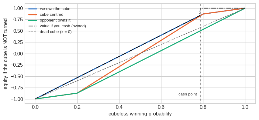
Equations 5–7 are linear in \(p\), so they run straight past the values a game can actually pay. GNU Backgammon and BGSage instead pin the live-cube equity at the four points where it is known — \(-L\) at \(p = 0\), \(-1\) at the take point, \(+1\) at the cash point, \(+W\) at \(p = 1\) — and interpolate linearly between them, flattening the outer segments to \(\pm 1\) under Jacoby. That is a substitution for equation (7), not an approximation of it.
It is also more accurate. On owned cubes the piecewise form reaches RMSE 0.0177 against 0.022–0.027 for the algebra, and its fitted indices sit close to the convention rather than scattering. raccoon/cube/janowski.py implements the piecewise form.
The bounds are provable, so they should never be fitted
If you double and your opponent takes, they took because taking beat passing for them, so you collect less than \(+1\); if they pass you collect exactly \(+1\). No doubling line pays more than a point. Undoubled you cannot collect more than the natural size of the win. So
\[-L \;\le\; E \;\le\; \max(1, W) = W\]
and under Jacoby with the cube centred this tightens to \(\pm 1\), since an undoubled gammon counts one anyway. The measured rollouts respect it. The piecewise form satisfies it by construction — both the dead and the live branch lie inside the bounds, so any blend of them does too — which is a second reason to prefer it over the algebra, which breaks the bound by up to a full point. We pin this as a property test rather than enforcing it with a clamp, so a change that breaks it fails loudly instead of being silently patched over.
Floor \(W\) and \(L\) at one point
Not a defensive nicety; the labels violate it. Variance reduction reports corrected means rather than counts, so a rare outcome can come back very slightly negative, and \(W = 1 + (P_{gw} + P_{bgw}) / P_{win}\) divides that by a win probability that can be minute. Across this benchmark that produces 550 rows with \(W < 1\), ten of them below zero, and a worst case of \(-5.29\) — which would put the take point and both envelope endpoints through the floor. A win cannot be worth less than a point. Flooring inside compute_wl repairs every consumer at once.
What should the implementation look like before any tuning? → Piecewise interpolation, bounds as a test rather than a clamp, and \(W, L \ge 1\). All three are free: no parameter, no fitting, no benchmark needed.
How to measure it
Cube models are usually argued about rather than measured, because the references are hard to come by. This benchmark has them — but most of its entries cannot judge a Janowski variant, and it takes two fields to tell which can.
It takes two fields to identify a measurement
eval_level records how a reference was produced; tier records how much effort the decision earned. Neither is sufficient alone, because BGSage gives truncated rollouts the same Rollout label as full ones. Crossed:
| reference | tier |
eval_level |
cube entries | rolled-out candidates |
|---|---|---|---|---|
| played to completion | rollout |
Rollout |
282 | 33,395 |
| truncated at 3-ply | 3T |
Rollout |
418 | 9,241 |
| 3-ply search | 3P |
3-ply |
1,496 | — |
Only the first row is an observed average. The truncated rollouts stop at a cubeful 3-ply evaluation that calls Janowski at its own leaves, and the 3-ply references are that same search all the way down — so scoring a Janowski variant against either is scoring it partly against itself.
The bias does not show up where you would look for it. Pooled cube PR barely moves — 2.353 over all references against 2.259 over the measured ones — because the contaminated groups pull in opposite directions: the model scores an implausible 0.649 against the 3-ply references it half-agrees with, and 7.726 against the truncated ones, which are the hardest decisions in the benchmark. The level looks fine. What breaks is every comparison made on it:
| references | baseline | one refitted index | paired gain |
|---|---|---|---|
| all 2,196 entries | 2.353 | 1.185 | +1.167 ± 0.271 |
| the 282 measured ones | 2.259 | 2.130 | +0.128 ± 1.242 |
Deeper cubeful search sees cube value a static evaluation cannot — market losers, mostly — so a larger \(x\) lets a 0-ply model imitate a 3-ply one. Refitting against search-derived references buys depth, not accuracy, and it does not survive contact with a real payoff.
The checker rollouts are the instrument, not the cube decisions
The benchmark’s cube entries look like the natural place to test a cube model, but only 282 of them are measured, and a cube decision structurally cannot separate the three formulas — it compares two locations at a time. The checker candidates can. Every one carries a measured cubeful equity beside the cubeless probabilities for the same position, and the parent decision records where the cube sat, so each formula is testable on its own against 33,395 observations.
Two properties of these positions carry into every conclusion below. They are post-move positions, so the opponent is on roll — the formulas do not model whose turn it is, so we evaluate from the on-roll player’s side and negate. And the cube decisions taken during each rollout come from a bot that also uses Janowski, so these measure equity under Janowski-quality cube play rather than optimal cube play.
The references have a noise floor
Every rolled-out candidate carries a standard error, so the benchmark can be asked how well it knows its own answer:
Across 5,651 rolled-out decisions the median standard error on the gap between the best move and the runner-up is 0.0033 of a point. 32% of those decisions have their best move within one standard error of the second-best, and 51% within two.
That noise is fixed and identical for every engine scored, so comparisons stay fair. But it puts a floor under achievable PR, and it is why a near-parity engine cannot be separated on move accuracy alone — a third of the closest decisions in the benchmark do not have a knowable right answer.
Compare like with like, or the model is charged for an option
Janowski’s formulas give the no-double equity — what a position is worth if the cube stays put — while a rollout reference always includes the option to double. Comparing the two directly charges the formula for an option it was never asked to price. Since these are post-move positions the option belongs to the opponent, so the matching quantity is \(\min(\text{ND}, \max(\text{DT}, -1))\): a minimum over their choice, a maximum over ours. Getting that backwards inflates the centred error by half. Four positions checked by hand in GNU Backgammon confirm the distinction — its No double line reproduces cl2cf_money closely and its optimal line matches the rollout.
Can Janowski be measured with what we already have? → Yes — on 33,395 observed cubeful equities, spanning all three cube locations, at zero play cost. But only an eighth of the benchmark’s cube entries can judge it, and a pooled score hides that: the level looks normal while every comparison built on it inflates.
What the measurement says
| formula | cube location | n | bias at 0.68 | RMSE at 0.68 | best \(x\) | RMSE there |
|---|---|---|---|---|---|---|
| \(E_O\) | we own the cube | 14,813 | +0.0007 | 0.0179 | 0.710 | 0.0177 |
| \(E_C\) | cube centred | 10,677 | +0.0135 | 0.0430 | 0.925 | 0.0307 |
| \(E_U\) | opponent owns it | 7,905 | +0.0025 | 0.0162 | 0.720 | 0.0155 |
\(E_O\) and \(E_U\) are right, and the published constant is right for them. Bias under 0.003 of a point across 22,718 positions, RMSE under 0.018, and freely fitted indices of 0.71 and 0.72 — close to each other and close to 0.68, which is what a genuine property of the position should look like. Refitting moves their RMSE by about 1%.
\(E_C\) is the outlier. Nineteen times the bias, more than twice the RMSE, and it wants 0.925 — a nearly perfect cube. Even there it stays worse than the other two are for free.
An independent check that the method is sound rather than the model being uniformly bad: let the index float against the take/pass line alone, told nothing about what it should be.
Across all 282 measured cube positions the take/pass index comes out at 0.700, against GNU Backgammon’s published 0.68. Within pure races it comes out at 0.515, against GNUBG’s documented 0.60 race constant.
The measurement reproduces both published constants without being told either.
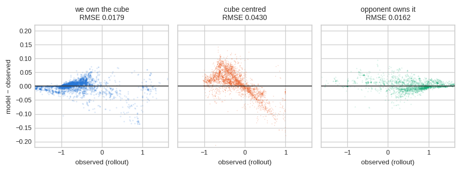
Averages hide where the failures are. Binning the same errors by observed equity, with intervals clustered on the checker decision — candidates within one decision are the same position played different ways, and clustering roughly doubles the intervals against treating them as independent:
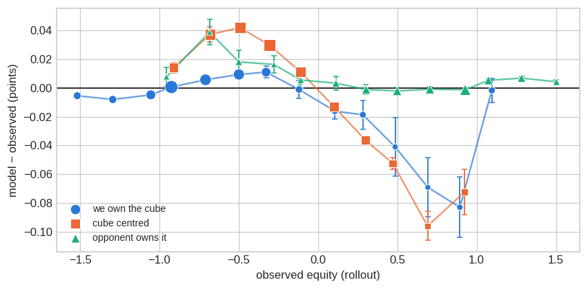
\(E_U\) is correct wherever it has weight — on zero from about \(-0.2\) equity upward. \(E_O\) is correct until the position is nearly won, then sags through the band where a cashing decision is live and snaps back above \(+1.0\). That band is thin, which is why the aggregate barely notices it. \(E_C\) is wrong in both directions — positive when the position is losing, negative when it is winning, crossing zero near even equity. A residual that changes sign cannot be removed by any constant, any index, or any offset.
The \(E_O\) sag has a mechanism worth naming, because it is a modelling choice rather than a measurement question. The model blends a dead branch with a live branch in fixed proportion, \((1-x)E_{\text{dead}} + xE_{\text{live}}\). As a position approaches its cash point the live branch has reached its ceiling of \(+1\) while the dead branch is still only \(2p-1\), so the blend drags the answer down by roughly \((1-x)\) times the gap between them. But a position near its cash point does not need future cube efficiency — you double and your opponent passes. A fixed weight is defensible in the middle of the range and not near the boundary.
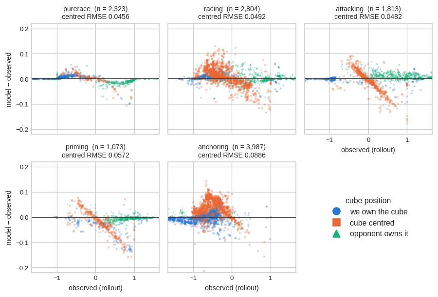
Where is the model weak? → Only in the centred formula, and everywhere in its range rather than in one position type or one game plan. The other two are correct at the published constant.
Why we are not acting on the centred index
A centred cube fits at 0.925 — almost a perfect cube. The result is robust: it survives clustered bootstrapping, disjoint halves of the games, and every formulation of the Jacoby handling we tried, and it reproduces on the benchmark’s own cube entries, which need no perspective flip at all. It is also the case where \(x\) matters most. And we still cannot explain it.
Two honest readings remain, and this data cannot separate them. Either an initial double really is more efficient than a redouble — both players can pick their moment, and a full ladder of recubes lies ahead — or the centred formula is missing something structural that \(x\) absorbs. The second is the better bet given the sign change above, since no constant can produce one.
What settles the practical question is that adopting it buys nothing.
The index is read for move selection, not for takes
Everything above is an estimation metric: every candidate weighted equally, scored on how close the model lands. That is not how the parameter earns its keep. Over 500 games the benchmark asks:
| question | times in 500 games | relative frequency |
|---|---|---|
| which move? (every turn) | 14,693 | 22.5× |
| should I double? (every turn with cube access) | 2,189 | 3.4× |
| should I take? (only when actually doubled) | 653 | 1.0× |
So the index is read for move selection roughly 22 times as often as for a take decision — and move selection only cares about the ranking of candidates within one position, where an error common to all of them cancels. A change can look valuable on RMSE and be worth nothing here. On the 5,695 measured decisions that offer a real choice:
| setting | picks the best move | mean cubeful equity lost |
|---|---|---|
| published x = 0.68 | 88.0% | 0.00053 |
| centred 0.925, owned 0.68 | 87.6% | 0.00060 |
| one refitted index (0.800) | 88.0% | 0.00053 |
Retuning moves this by a fraction of a percentage point, and the centred refit makes it slightly worse. There is no case for shipping it.
Should the centred index be changed? → No. It is a real and unexplained feature of the data, but acting on it costs accuracy where the parameter is actually read. Keep 0.68 and record the anomaly as open.
exp024, re-scored
Hypothesis. Janowski’s functional form is adequate and its published cube-life index is simply mis-set: re-fitting \(x\) recovers the cube-decision error that \(x = 0.68\) leaves.
Primary metric. Cube PR on the BGSage money benchmark — mean equity thrown away per decision, times 500 — restricted to the 282 positions whose references were played to completion, n = 432 sub-decisions, fed the benchmark’s own reference probabilities so the net’s evaluation error is out of the comparison. Variants are fitted on half the games and confirmed on the held-out half, and compared to the baseline paired.
| variant | cube PR | paired vs baseline | coherent? |
|---|---|---|---|
| \(x = 0.68\) (published) | 2.259 ± 0.488 | — | yes |
| 0.68 contact / 0.60 race | 2.228 ± 0.489 | +0.031 ± 0.112 | yes |
| one refitted index | 2.130 ± 1.140 | +0.128 ± 1.242 | yes |
| refitted per cube state | 1.306 ± 0.326 | +0.953 ± 0.528 | no (93% violations) |
| 0.68 plus a fitted shift | 2.138 ± 0.477 | +0.121 ± 0.190 | yes |
| \(x = 0\) (dead cube) | 5.566 ± 1.657 | -3.307 ± 1.647 | no (94% violations) |
| \(x = 1\) (live cube) | 6.680 ± 1.950 | -4.422 ± 2.058 | yes |
Nothing beats the published constant. The two fitted variants land about 0.12 lower with intervals many times that wide, the race split is inside noise, and the dead and live envelopes are far worse — which is the sanity check that the model is doing real work between them.
The coherence gate matters more than the PR column. For any one position \(E_O \ge E_C \ge E_U\) must hold: owning the cube cannot be worth less than it being centred, which cannot be worth less than the opponent owning it. Nothing in the fitting enforces that, because each entry is either centred or owned, so the three lines are fitted on disjoint position sets. The per-state fit scores best on PR and drives the owned-cube index to 0.42 against the 0.71 the equity data gives, inverting the ordering on 93% of positions. PR cannot see that, because each scored decision involves only one cube location. A mis-set constant cannot produce an impossible ordering; a mis-specified form can.
Power, stated rather than assumed. 432 sub-decisions cannot resolve a small change: the paired interval on the refitted index is ±1.242, so this test would miss anything under about a point of PR. It is a null in the sense of no evidence of benefit, not proof of no effect. The move-selection comparison above, at 5,695 decisions, is the better-powered instrument and agrees.
Where Raccoon’s own evaluations land
| probabilities | cube PR (n = 432) |
|---|---|
| benchmark reference (the model alone) | 2.259 ± 0.488 |
| Raccoon exp018/ep22 | 2.684 ± 0.622 |
| GNUBG 0-ply | 2.658 ± 0.638 |
Raccoon’s net and GNUBG at 0-ply are indistinguishable on cube decisions, and both sit a little above what the model reaches on perfect probabilities — the cost of evaluation error rather than of cube modelling.
Is the cube-life index mis-set? → No. Against references that are measurements, no variant beats \(x = 0.68\) (best: one refitted index, +0.128 ± 1.242 paired, n = 432). The earlier +3.206 came from references produced by a search that uses Janowski at its own leaves.
What Raccoon will build
Raccoon has no cube at all today. The shipped net already emits the six-outcome distribution the cube needs, raccoon/cube/janowski.py is written and tested, and nothing in the playing path references it. This is the specification for closing that gap, in the order the measurements above say to do it.
The model, settled. Piecewise dead/live blend; \(x = 0.68\) for contact and \(0.60\) in races; one index for all three cube locations, never one per location; \(W\) and \(L\) floored at 1; the \([-L, W]\) bound as a test.
The inputs, all present. RaccoonNet.value_probs6 → janowski.probs6_to_cumulative5 → janowski.cube_action. No model work is needed; the value head has carried the six-outcome distribution since exp018.
Cube-aware checker play comes first — not the double/take decision. Ranking afterstates by cubeful rather than cubeless equity in raccoon/train/lookahead.py is where the model gets read 22 times as often, and the prize is already measured: a perfect cubeless player throws away
PR 0.336 ± 0.042 on the cubeful metric, with cubeless-best and cubeful-best differing on 992 of 14,693 decisions (6.8%). It concentrates exactly where the cube is most alive — PR 0.553 with the cube centred against 0.145 when the opponent owns it — and is nearly absent in pure races (0.046).
Then the cube decision itself, via cube_action at the top of a turn, and the plumbing it needs: cube_value and cube_owner threaded through the play loop, raccoon/eval/arena.py and raccoon/protocol/rgp.py, none of which have any concept of a cube today.
How to score each. Cube decisions on the 432 measured sub-decisions, knowing that is underpowered for anything small. Move selection on the 33,395 clean candidates, by picks-best-move rate and mean cubeful equity lost — the metric that matches the frequency with which the parameter is read.
Explicit non-goals. Do not tune \(x\) against 3-ply references. Do not score a cube change on take decisions alone. Do not chase the centred index until there is a reference not generated by a 0.68 policy.
What this page does not establish
- The population is not the target. These are 500 games of one engine playing itself. An index fitted here describes how efficiently that bot uses the cube, on the positions its own style produces.
- The references are not optimal cubeful equity. The payoff is empirical, but the cube decisions taken during each rollout come from a bot that also bottoms out in Janowski. Policy error can only lower realised equity, so this understates what a better model could reach rather than overstating it.
- The benchmark is played under Jacoby, and Raccoon’s target is not. The project aims at money game without Jacoby, as the stepping stone to match play (
goal.md). Jacoby zeroes gammons while the cube is centred, so on those positions the reference engine plays boldly — it leaves the cubeless-best move 25.2% of the time against 10.7% with the cube owned, giving up five times as much cubeless equity and trading away gammon wins as readily as it accepts gammon losses, since the rule makes both worthless. That is 38.5% of the benchmark’s checker decisions, and it taints the labels rather than just the target: the rollout continuations behind them were played bold too. Regenerating without Jacoby means rebuilding every tier from new games, so we report the Jacoby-clean owned-cube subset alongside the full number instead. - Nothing here transfers to match play beyond that: score-dependent take points, no beavers, and Janowski in match-winning-chance space are all uncalibrated here.
- No position is observed at two cube locations, so the ordering constraint is a model check and can never be validated against data.
- The benchmark’s cube positions are selected for being non-trivial, so an index fitted on them is tuned for close decisions and should not be quoted as a general-purpose constant.
- Coordinate descent on a grid finds a coordinate-wise minimum, not a certified global one.
Still open
- The centred index. Two readings, no way to separate them here; it needs a reference not generated by a 0.68 policy.
- Whether an index per cube value is real. A centred cube is always a 1-cube here, so cube value and cube location tell the same story and cannot be told apart.
- Volatility measured rather than proxied. Janowski derives \(x\) as inversely proportional to volatility, and it can be measured directly — the spread of the 0-ply value over the 21 next rolls, reusing
raccoon/eval/luck.pyand the roll table inraccoon/search/expectimax.py. A cheap proxy does not work: the residual correlates with contact at only \(-0.15\), with no monotone trend, which is precisely why the direct measurement is the experiment worth running. - Cubeful search. GNUBG does not use the closed form as its cube engine — it uses it as a leaf evaluator inside a search that makes cube decisions at every node. The gap that refitting appeared to close against 3-ply references is that search, and running it is the principled way to close it.
References
- Rick Janowski, Take-Points in Money Games (PDF) — the cube-life index, equations (5)–(7) for the three cube locations, the refined model of Appendix 2, and the Jacoby factors of Appendix 3.
- Keeler and Spencer, Optimal Doubling in Backgammon (1975) (online) — the continuous model behind the live-cube take point.
raccoon/cube/janowski.py— the model, ported from the paper and cross-checked against its worked examples and against GNU Backgammon.experiments/pipeline_exp024.sh— every number on this page, reproducible end to end.